Why is this a prelude?

I was in the final stages of writing a blog post about particle interactions and Feynman Diagrams when I decided to pause for a bit and write this instead. I had structured that article such that I present the fundamental interactions described by the Standard Model in detail and then I would give an introduction to Feynman diagrams and provide example Feynman diagrams for all the interactions I had already presented. The first problem I faced was that the post got quite long quite quickly and I hadn't even started tackling Feynman diagrams yet!

My solution to this was to do something I had done previously and that was to split the article up into two parts (I did that with part 1 and part 2 of this series), with the second part covering Feynman diagrams and giving examples.

However, as I wrote more and more about interactions, I realised the article felt quite dry without any visual aids. It also occured to me that I really should say everything I'd like to say about each interaction in that interaction's section in the article. And this should include the Feynman diagrams associated with this interaction!

So what I decided to do was to first write and release this prelude article introducing the readers to Feynman diagrams and giving brief examples about them, with more detailed examples to come in the next article. At the time of writing this, the main part 3 of this series is almost completed with just the Feynman diagrams yet to be added to each interaction. My goal is to hopefully release that within a few days of this short prelude being published. As this is essentially meant to be a crash course on the topic, let's get started without further ado!

What are Feynman diagrams?

Feynman diagrams are a way to graphically visualise particle interactions. And indeed, they are incredibly flexible in what can be done with them and they, in fact, represent all the maths behind every interaction fully. Every line and vertex in the diagram represents a term in the Lagrangian of the interaction. The mathematical description of the interactions we're going to consider, however, is very much out of the scope of these articles.

Feynman diagrams represent interactions in a way governed by these guidelines:

• Particles are represented by world lines in time and space.
• Time flows along the horizontal axis from left to right.
• Space is represented in the vertical direction (one or all of the 3 spatial dimenstions).
• Normal matter (as opposed to antimatter) particles have arrows pointing forwards in time.
• Antimatter particles have arrows pointing backwards in time.
• Photons are represented by wiggly lines (a wave) without arrows.
• Gluons are represented as a 2D helix shape (like a screwdrive), as we'll see below.
• Other bosons are represented as dashed lines.
• Points where lines meet are called vertices and conservation laws must be obeyed before and after them.

For the purpose of this, we consider antiparticles to be moving backwards in time. The reasons for this relates to CPT symmetry, which I briefly discussed in my article about symmetries in physics, and is beyond what we'll talk about here.

Consider this example to demonstrate how we're representing time and space here. Two electrons are seperated by a certain distance and they start moving towards each other. Say we define the positive direction to be the direction in which the first electron moves. This means that the second electron must move in the negative direction. This is normal and we might expect to represent this on a space diagram with two lines going opposite each other. Now consider also time. Both electrons are going forwards in time. This means that on a time diagram, we might expect them to be represented by two parallel lines pointing in the same direction. Combine these two representations and we should see diagonal lines across the spacetime diagram; something like this:

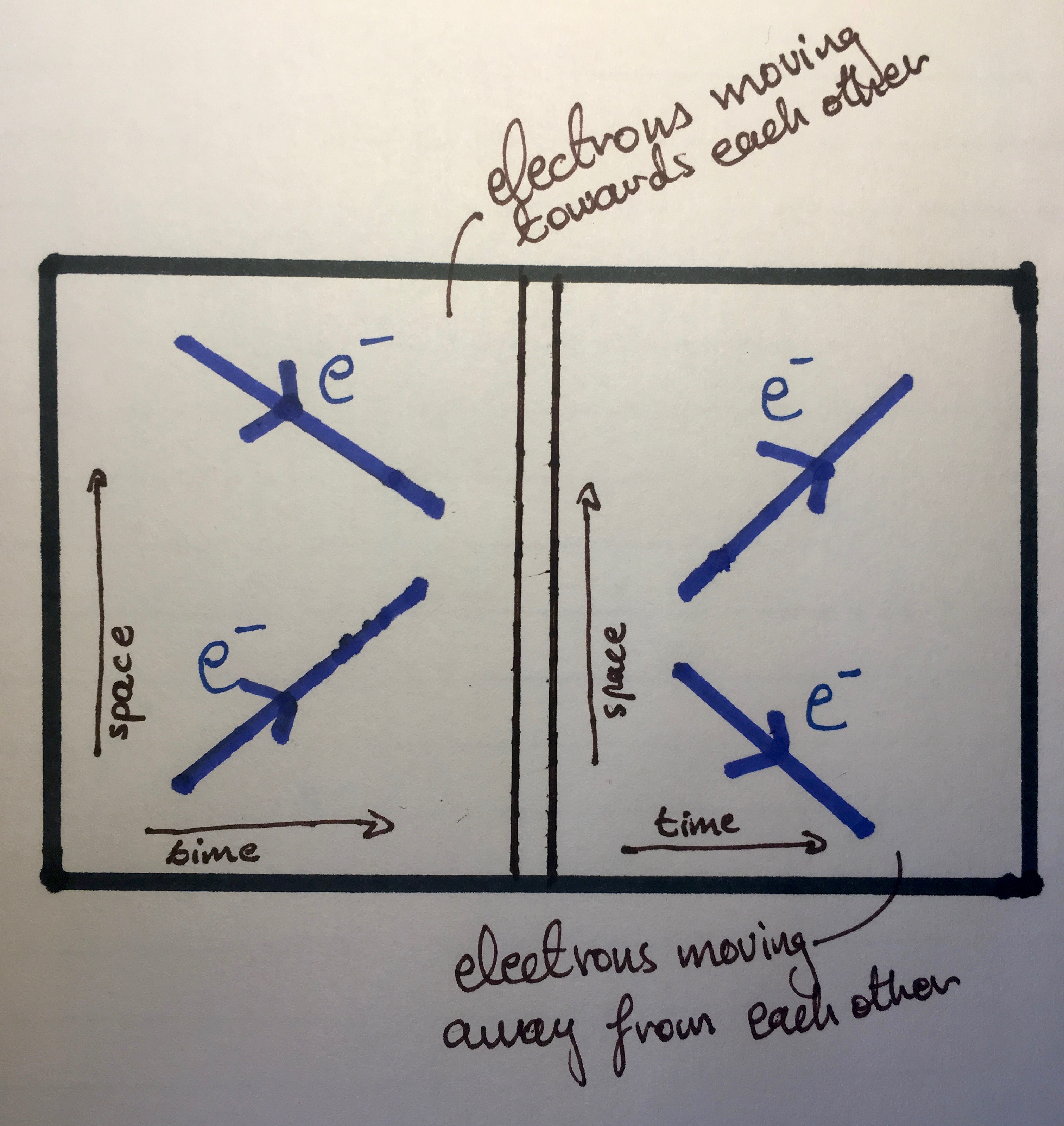
Left: Electrons moving towards each other. Right: Electrons moving away from each other. Notice how we see diagonal lines despite the fact that they are moving in a straight line in space.

Regarding the guidelines

Note that I said that these were guidelines. Indeed these are not set properties of Feynman diagrams as, for instance, some people prefer to use the horizontal axis for space and the vertical axis for time rather than vice versa. I have also seen weak bosons (W⁺, W^-, Z⁰) sometimes represented as wiggly lines as opposed to dashed lines. The important thing is to either be consistent or define your axes and so on for every diagram. Sometimes it is more favorable to draw the Feynamn diagram with time on the vertical axis and space on the horizontal axis in terms of clarity. For the purpose of these articles, I will be following the guidelines set above (time horizontally, space vertically), unless explicitly stated otherwise on the diagram.

Rotating and twisting Feynman diagrams

One of the brilliant features of Feynman diagrams is that once you have the Feynman diagram for a particular interaction, you would be able to twist certain vertices or rotate the diagram to arrive at diagrams for other less probable interactions. We will see this in action as we consider examples here and in the main part of the article.

Examples

We'll have a look at some examples of Feynman diagrams for some simple interactions to illustrate the guidelines above, without giving too much detail about the interactions themselves as that's coming in the main part.

Note that you should be able to apply conservation laws to verify that the quantum numbers involved in each interaction are balanced. For your reference, I will provide the tables containing the quantum numbers associated with each fermion (quarks and leptons) here:

Quarks

	Symbol	Upness	Downness	Charm	Strangeness	Topness	Bottomness	Charge
Up Quark	u	1	0	0	0	0	0	2/3
Down Quark	d	0	1	0	0	0	0	-1/3
Charm Quark	c	0	0	1	0	0	0	2/3
Strange Quark	s	0	0	0	-1	0	0	-1/3
Top Quark	t	0	0	0	0	1	0	2/3
Bottom Quark	b	0	0	0	0	0	1	-1/3

Table showing quantum numbers associated with quarks.

Leptons

	Symbol	Electron Lepton Number	Muon Lepton Number	Tau Lepton Number	Charge
Electron	e-	1	0	0	-1
Electron Neutrino	νe	1	0	0	0
Muon	μ-	0	1	0	-1
Muon Neutrino	νμ	0	1	0	0
Tau	τ-	0	0	1	-1
Tau Neutrino	ντ	0	0	1	0

Table showing quantum numbers associated with leptons.

Example 1: Pair Annihilation

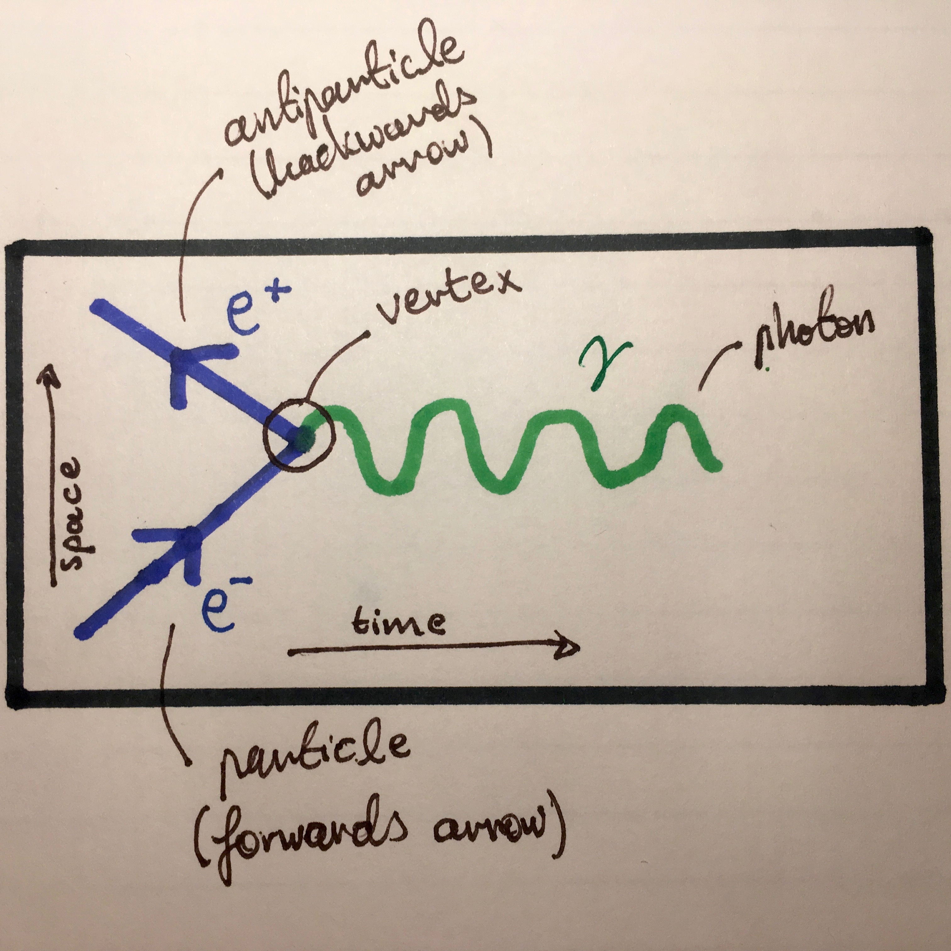
Pair annihilation Feynman diagram. Notice that we can apply conservation laws before and after the vertex to make sure they are obeyed. Relevant quantum numbers here are charge and electron lepton number.

Example 2: Photon Absroption

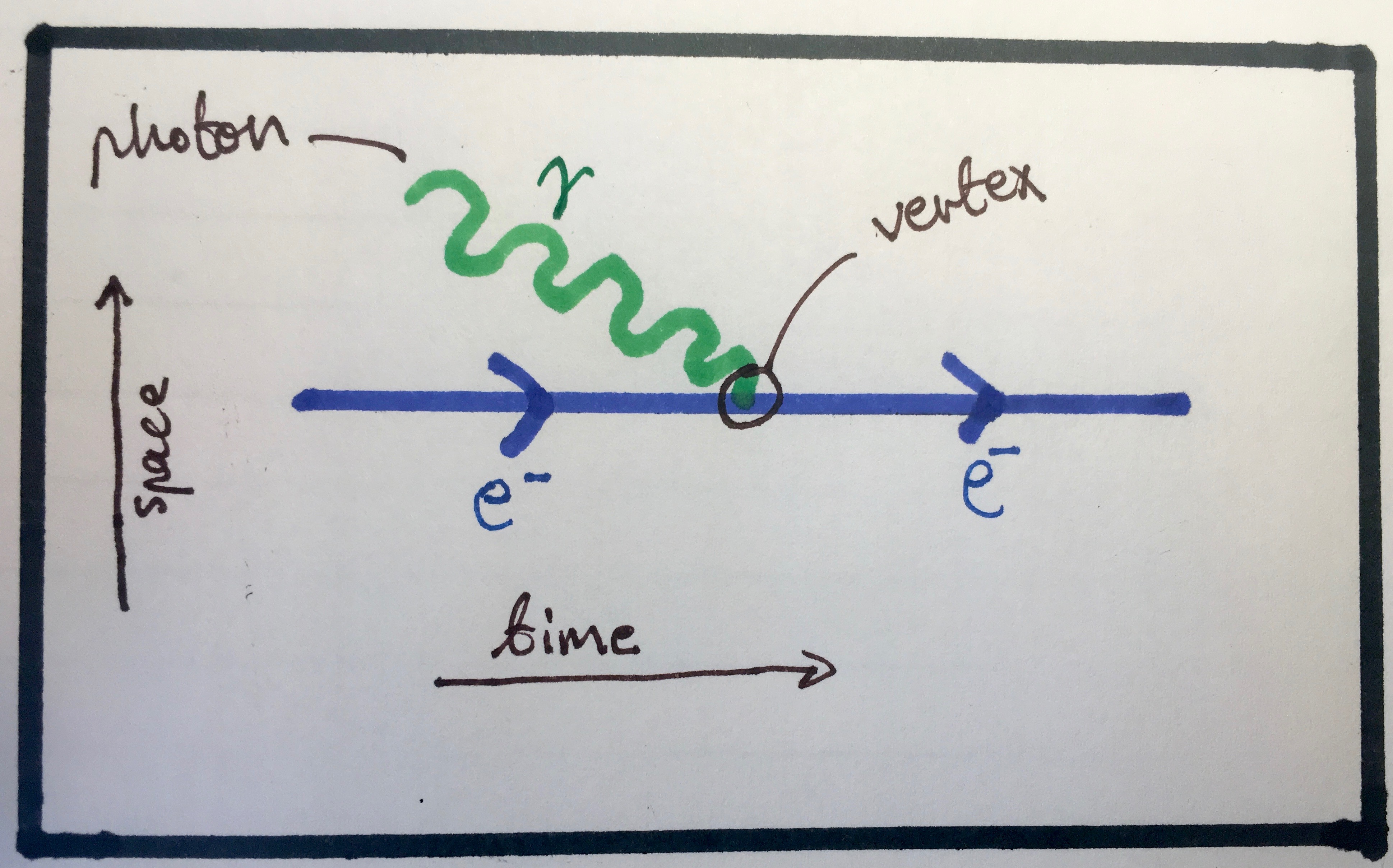
Feynman diagram representing an electron absorbing a photon, moving to a higher energy level.

We can reflect this diagram to arrive at essentially the opposite interaction, where an electron emits a photon and moves to a lower energy level.

Going forward, I will be omitting the extra labels on the diagrams, like the vertices and so on, to show you the diagrams as how we'd usually draw them, unless absolutely necessary.

Example 3: Photon Emission

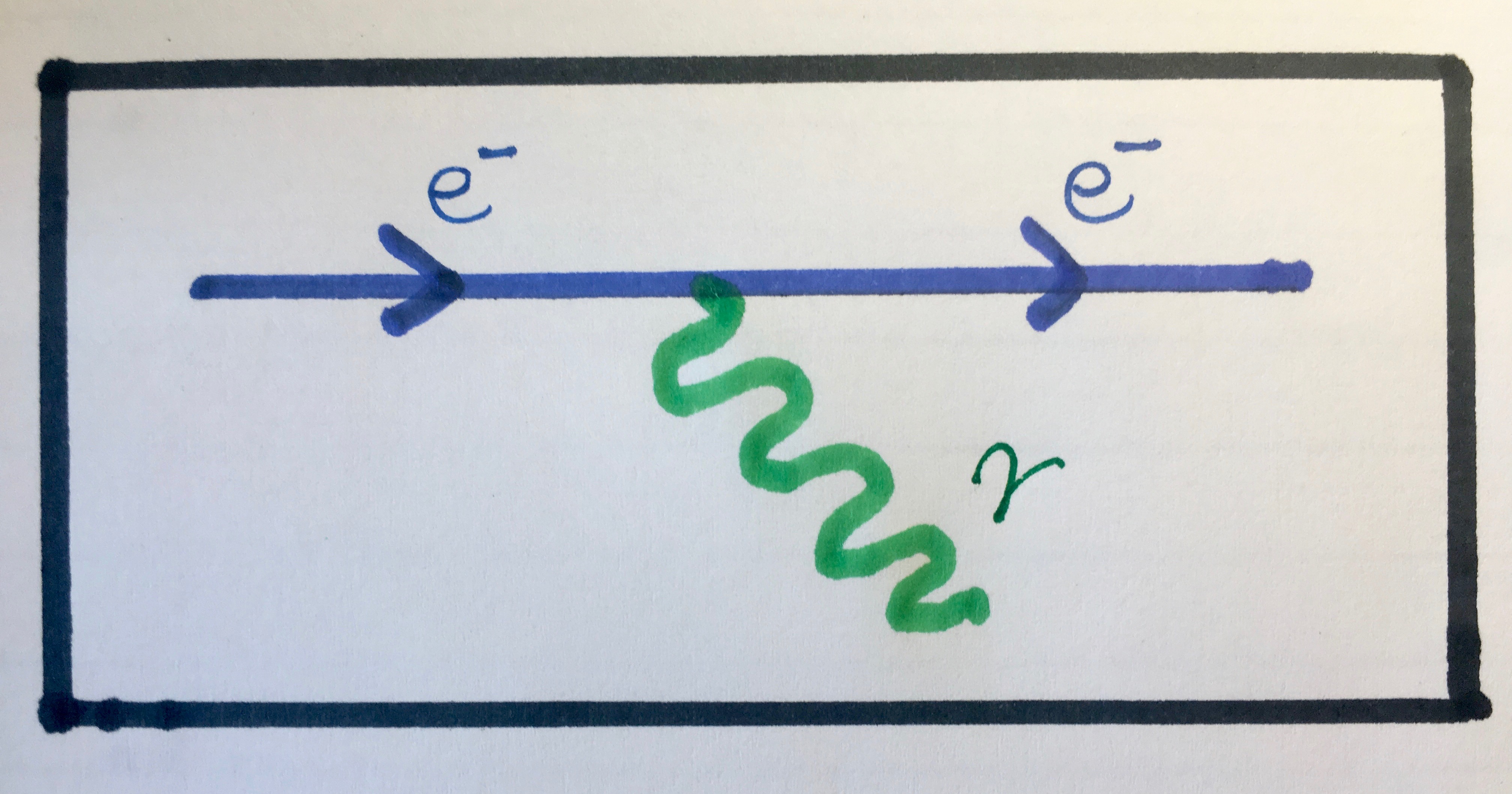
Feynman diagram representing an electron emitting a photon. Notice that you can arrive at this by reflecting the previous diagram showing photon absorption.

Example 4: Gluon Emission

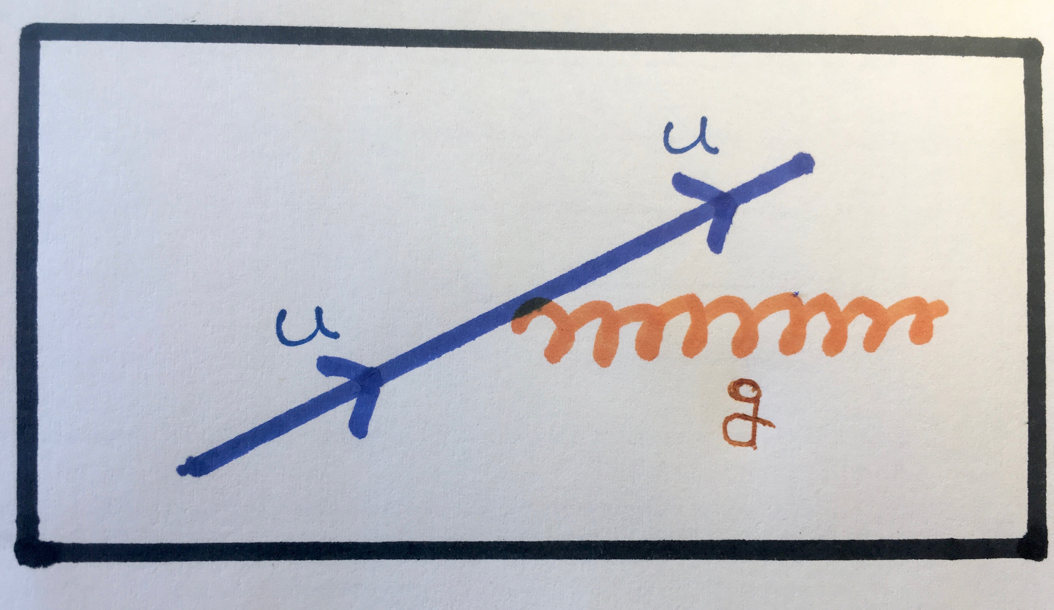
Feynman diagram representing an up quark emitting a gluon and, as such, changing its colour charge, as described here: Colourful Quantum Chromodynamics.

Example 5: Gluon Exchange

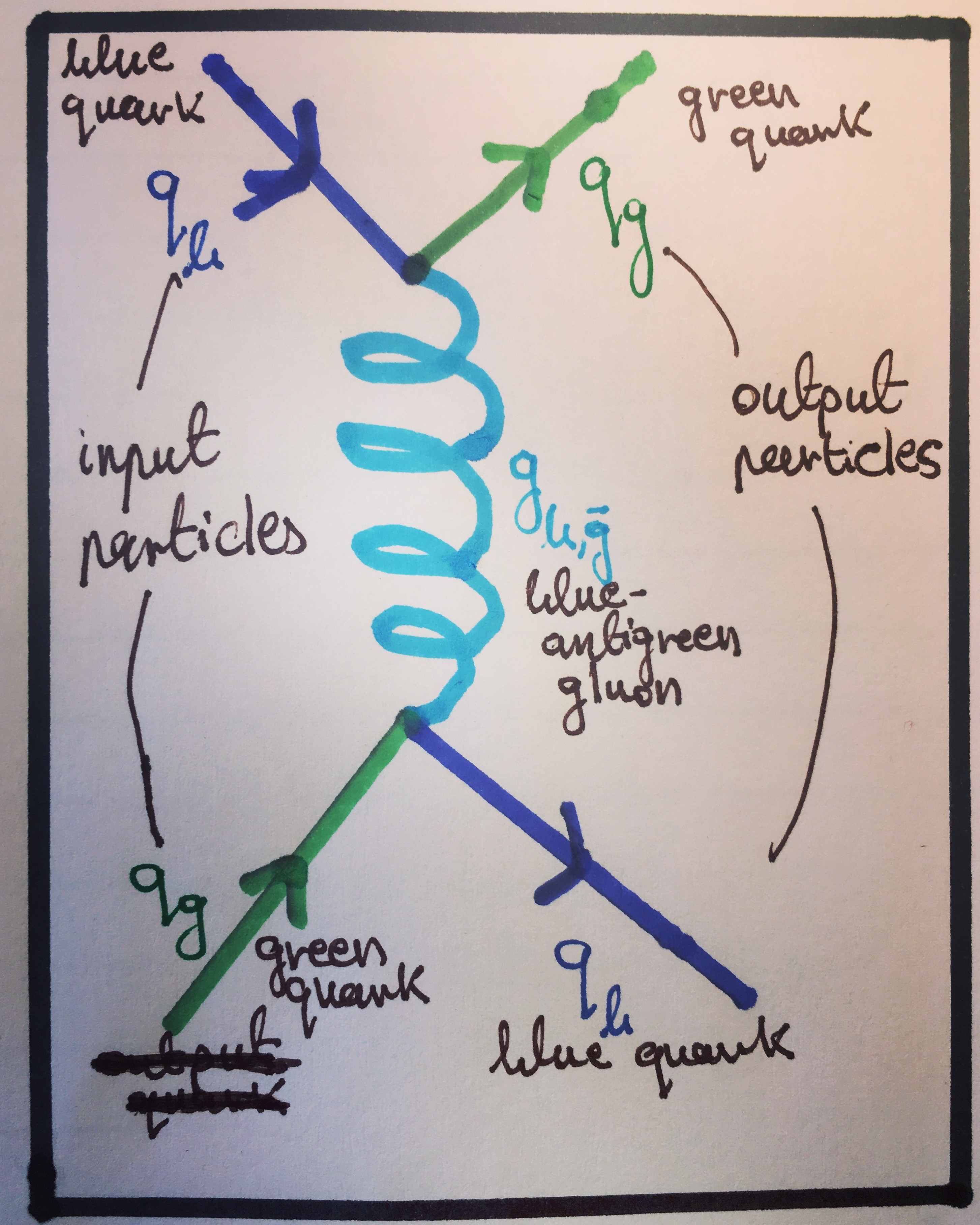
Feynman diagram showing the process of gluon exchange between two quarks which, when coupled with a third quark results in quark confinement inside a baryon. This process is also discussed in detail in the previous part of this series: Colourful Quantum Chromodynamics.

If you have read the last part of the series, see if you can check if colour charge is conserved across the vertices shown in the last example.

Example 6: Beta Decay

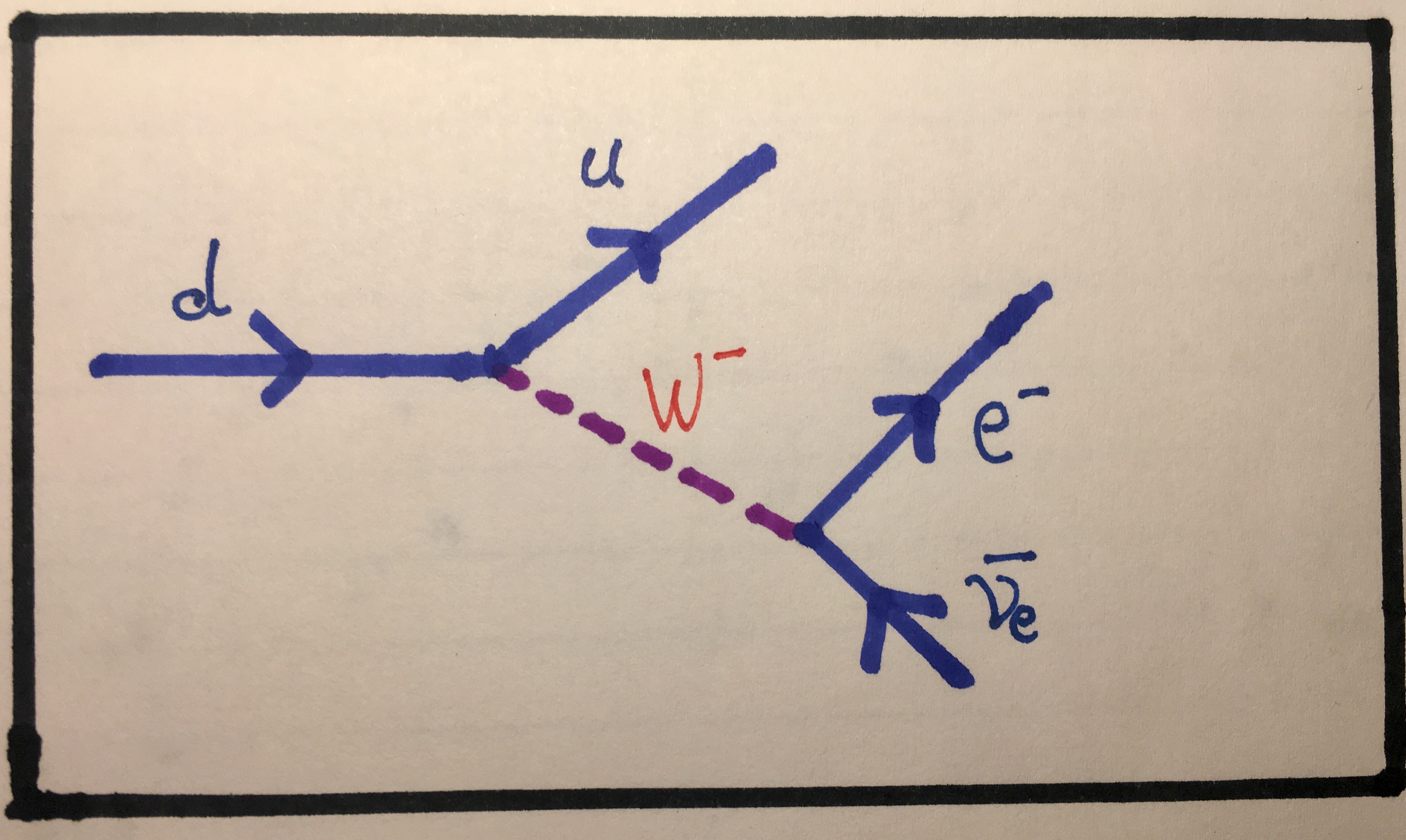
Feynman diagram showing the process of beta decay. Notice that a W^- boson is involved here. This implies that this interaction occurs through the weak nuclear interaction. This is one of the most important interaction we're going to consider in part 3 and is described briefly below.

We've discussed before, in the article about symmetries, how the weak interaction does not conserve quark flavour. And, indeed, in this interaction, we can see this happening. Across the first vertex, the upness and downness symmetries are not obeyed as the flavour number of the quarks is not balanced. In order for this to occur, a weak boson, specifically a W⁺ or a W^- as the quarks are electrically charged, must be emitted by the starting quark. In this case, a W^- boson is emitted in order to conserve charge. The W^- boson then decays into an electron and an antielectron neutrino (we'll look into this in more detail in the main article). You can confirm that electron lepton number is conserved across the last vertex as the antineutrino has the opposite electron lepton number to the electron. Notice also that because the antineutrino is an antiparticle, it has an arrow pointing backwards. Try to confirm also that charge is conserved across the first vertex and then across the second.

Conclusions

I hope I have demonstrated enough of the properties of Feynman diagrams for you to be able to dive straight into the main part of the article where we'll be discussing many more examples of these interactions and in more detail.

Personal note about Feynman diagrams

I've only relatively recently started learning about Feynman diagrams in university and I was absolutely fascinated by them. I believe this is undoubtedly related to my likeness towards symmetries, which I have expressed before in Symmetries: The Beauty in Physics. I think I saw these Feynman diagrams as a way of visualising these symmetries, in a way.

I was so fascinated by them, in fact, that I decided to augment the app about the Standard Model that I have been building (simply entitled The Standard Model) to provide functionality to automatically draw Feynman diagrams for interactions provided by the user. I think that without this feature, the app will definitely have been lacking something. I have not released this app yet as it is still a work in progress. However, I do have preliminary Feynman diagram drawing functionality ready. If you're interested, please feel free to read more and look at screenshots here.

Closing remarks

The main part of the article is almost complete and hopefully, I expect to release it within the next 2-3 days.

I hope you have enjoyed reading this and have found it informative! I will make sure to update this article with a link to the main part when it is published. Please feel free to leave a comment just below if you have enjoyed something in particular about this or would like something done better next time. Your feedback is always very much appreciated and will help to improve the blog. You can also contact me through the website or send me a tweet.

Thank you!

UPDATE (28/05/2017): Slightly belated, however the main section of this part is now live. Read it here: Interacting Particles.