Welcome back to Waves!

I've not put up a post about waves in a while, but I'm back to writing and have a few more posts in this series planned for the next few weeks! If you're new to the series, feel free to start at Waves I, which discusses the wave equation.

This part will not be following on directly from the previous part, like other parts do. Instead, all you really need to have read is what's discussed in Waves I and some bits from Waves II, where I introduce the concept of a constant shape travelling wave. In this article, I will cover solving the wave equation by seperation of variables, and getting a standing wave solution.

I will also assume you have an understanding of solving second order ordinary differential equations (not partial though; we'll go through that).

I will start by introducing some simple solutions to the wave equation, then move on to finding the standing wave solutions (the most general solution).

Solutions to the wave equation

Wait, where's the wave equation?! We derived the wave equation for waves on a string in Waves I to be:

$$\frac{\partial^2y}{\partial x^2}\frac T\rho=\frac{\partial^2y}{\partial t^2}$$

where $y$ is the vertical displacement of an infinitesimal string element, $T$ is the tension in the string and $\rho$ is the linear density of the string.

We won't really care too much about $T$ or $\rho$ in solving the the wave equation and since in Waves II we proved that $c = \sqrt{\frac T\rho}$, we can rewrite this as:

$$\frac{\partial^2y}{\partial x^2}c^2=\frac{\partial^2y}{\partial t^2}$$

Since the wave equation is a (partial) differential equation, there will indeed be many different solutions that can satisfy it. At the end of the day, the wave equation simply tells us how a wave, any wave, evolves with time and in space. Knowing that, we can make a very informed guess about the solution of the wave equation.

We assume we're dealing with a constant shape travelling wave on a string, the same kind we dealt with in Waves II. These are waves which retain a constant shape with time. Recall that in Waves II we proved a solution in the form $y = y(x\pm ct)$, where $y(x-ct)$ represents a wave moving in the positive-$x$ direction and $y(x+ct)$ represents a wave moving in the negative-$x$ direction.

We know the wave is periodic, and is.. well, a wave, so a sinusoidal solution would make sense. Consider this candidate for a solution:

$$y(x,t) = A\sin (k(x-ct)) = A\sin (kx-kct)$$

Two things to notice here are the amplitude, $A$, and the wavenumber, $k$. The amplitude is the maximum displacement that the string reaches in both the negative and positive directions. The wavenumber is a physical quantity that is necessary to be included here in order to make the argument of the $\sin$ function dimensionless. $\sin$ and $\cos$ (and the exponential function, $e^x$) must always take dimensionless arguments. The wavenumber is a quantity with units of $\textrm{length}^{-1}$ in order to balance the $\textrm{length}$ units of $(x-ct)$.

If you've read Waves IV, where we discussed power transmitted by a wave, this form will seem familiar to you. The form of solution we assumed there was:

$$y(x,t) = A\sin (kx-\omega t)$$

where $\omega$ is the angular frequency of the wave: $\omega = 2\pi f$ and $f$ is the frequency of the wave. And indeed $\omega$ here is equal to $kc$. Knowing that $c = f\lambda$, where $\lambda$ is the wavelength of the wave and that $k = \frac{2\pi}{\lambda}$, we can prove this:

$$ kc = \left(\frac{2\pi}{\lambda}\right)(f\lambda) = 2\pi f = \omega$$

Simple enough! We've now postulated that this could be a solution to the wave equation above. We need to prove this. We start by finding the second partial derivatives of this with respect to $x$ and $t$:

$$ \frac{\partial y}{\partial x} = kA\cos(kx-\omega t), \frac{\partial^2 y}{\partial x^2} = -k^2A\sin(kx-\omega t) $$ $$ \frac{\partial y}{\partial t} = -\omega A\cos(kx-\omega t), \frac{\partial^2 y}{\partial t^2} = -\omega^2A\sin(kx-\omega t) $$

Substituting these into the wave equation:

$$\frac{\partial^2y}{\partial x^2}c^2=\frac{\partial^2y}{\partial t^2}$$ $$ -k^2Asin(kx-\omega t) c^2 = -\omega^2A\sin(kx-\omega t)$$

We immediately see that we can cancel out $-A\sin(kx-\omega t)$ from both sides, to get:

$$k^2c^2 = \omega ^2$$

This is saying that our solution $y(x,t) = A\sin (kx-\omega t)$ does indeed satisfy the wave equation, if and only if the above condition involving $k$, $c$ and $\omega$ is satisfied. Taking the positive square root of both sides, we get $\omega = kc$, which is indeed the condition we defined when we were coming up with that solution.

So this solution is just fine! I also encourage the reader to prove that other sinusoidal functions are solutions to the wave equation. For example:

$$ y(x,t) = A\cos (kx-\omega t), $$ $$ y(x,t) = Ae^{i(kx-\omega t)} $$

are both solutions. You can prove this by following the same procedure we went through above for a $\sin$ solution.

But is this a general solution?

General solutions

We tested the above function, one of the form $y = y(x-ct)$, to check that it satisfies the wave equation. But what about the function that is moving in the opposite direction, $y = y(x+ct)$? Indeed we can have a solution of the form:

$$y(x,t) = y_1(x-ct) + y_2(x+ct)$$

where $y_1$ and $y_2$ are independent sinusoidal functions. Feel free to check that this is a solution.

This is a result of the Principle of Superposition (which I discussed before in an article about the double slit experiment), which states that when two (or more) waves propagate over the same medium, the resulting wave is the sum of the two waves.

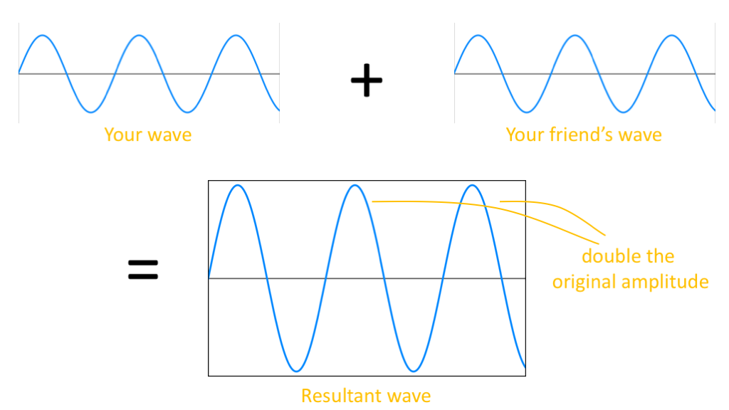
From Observers affecting reality? The Double Slit Experiment

Two waves add up to create a larger wave.

As a matter of fact, we can add up as many of these as we want and still have a solution which satisfies the wave equation:

$$y(x,t) = Ay_1(x-ct) + By_2(x+ct)$$

So how do we find a more general solution, one which can represent the addition of many waves? We will have to solve the wave equation analytically and use a partial differential equation solving technique like seperation of variables. When we do do that, we ought to expect our solution to be similar to this. But before we do that, let's discuss standing waves.

Standing Waves

Standing waves are waves which do not propagate through space, but rather individual elements in the wave move transversely (or longitudinally). In our case of the string, this means that the infinitesimal string elements move up and down a constant amount each period.

Imagine holding the end of a string which is attached to a wall at the other end. You start wiggling the string up and down, and travelling waves start to propagate through the string. Eventually the waves reach the end of the string that's fixed to the wall, and they reflect back towards you. What happens now? There are now two waves propagating through the string in opposite directions. A standing wave starts to form on the other end of the string as the reflected wave travels back and interferes with your wave (I covered interference before in the double slit experiment article). The standing wave keeps getting "longer" as more waves are reflected until eventually they reach your end of the string and you get a standing wave throughout the whole of the string (assuming you've been wiggling the string with a regular period and continue doing so when the reflected waves reach you). This is demonstrated here:

By LucasVB - Own work, Public Domain - Link - through Wikipedia

A standing wave. There are two waves propagating in this case, the red and blue waves visible in the background. Notice how the blue wave is moving to the right while the red moves to the left. The resultant wave, which is the black wave in the animation, is formed by the superposition of the red and blue waves at each point in time. The result is a wave that doesn't seem to be moving left or right, but rather has elements moving transversely.

We call the points where destructive interference happens nodes, and the points where constructive interference happens with maximum displacement antinodes. In the animation above, the red dots are where nodes happen (the string element there is completely stationary throughout the wave's period). Antinodes happen halfway between any two nodes (points where the wave looks "stretched" the most).

So how do we describe these waves mathematically? We need to find a solution general enough for this, so we use the seperation of variables method to do this.

Seperation of Variables

Seperation of variables is a well known method for solving some partial differential equations. By applying it to the wave equation, we can get a solution general enough to describe the phenomenon of standing waves.

Seperation of variables really has two key steps: 1) assuming that the solution is a product of functions of each of the variables involved ($x$ and $t$ in this case), and 2) recognising that two sides of an equation that each depend on only one variable must mean that both sides are equal to some constant (known as the seperation constant). The second step may not be entirely clear right now if you haven't used seperation of variables before, so let's go ahead and apply this to the wave equation.

The wave equation is:

$$\frac{\partial^2y}{\partial x^2}c^2=\frac{\partial^2y}{\partial t^2}$$

We're looking for a solution for $y$, so let's apply the first step and assume that the dependence of $y$ on $x$ and $t$ is seperate, i.e. $y$ is a product of a function of $x$, call it $X$, and a function of $t$, call it $T$:

$$ y(x,t) = X(x)T(t) $$

This is a candidate solution, like the one we had before. We can easily plug it into our wave equation, so let's do that. First find the second partial derivatives as before:

$$ \frac{\partial y}{\partial x} = \frac{dX}{dx}T, \frac{\partial^2 y}{\partial x^2} = \frac{d^2X}{dx^2}T $$ $$ \frac{\partial y}{\partial t} = X\frac{dT}{dt}, \frac{\partial^2 y}{\partial t^2} = X\frac{d^2T}{dt^2} $$

Let's plug this into the wave equation:

$$ \frac{d^2X}{dx^2}Tc^2 = X\frac{d^2T}{dt^2} $$

Let's divide both sides by $XT$ (to seperate variables)and move the $c^2$ to the other side as well:

$$ \frac 1X \frac{d^2X}{dx^2} = \frac 1T \frac 1{c^2} \frac{d^2T}{dt^2} $$

Since $c^2$ is a constant, what we have here are two functions of seperate indepedent variables ($x$ and $t$) on two sides of the equal sign. The only way this condition is satisfied is if both sides are equal to some constant. This is the second key step mentioned above. Assume this constant is equal to $-k^2$, where $k$ is the wavenumber discussed above (we'll prove the same condition later). And so we have:

$$ \frac 1X \frac{d^2X}{dx^2} = -k^2 = \frac 1T \frac 1{c^2} \frac{d^2T}{dt^2} $$

Consider each equation by itself:

$$ \frac 1X \frac{d^2X}{dx^2} = -k^2 $$ $$ \frac 1T \frac 1{c^2} \frac{d^2T}{dt^2} = -k^2 $$

What we have here are two second order ordinary differential equations. These differential equations will have more than a single solution, so for the purposes of finding a standing wave solution, we'll make another well educated guess about the form of the solution. In fact, later on when we study boundary conditions, we will be able to show that the general solution simplifies to the form we will try now.

Try a solution of the form:

$$ X(x) = A\sin (kx) $$ $$ T(t) = B\sin (kct) $$

Check that this solution does indeed satisfy the differential equations above! Some solutions will include a phase term here (which would make the solution look like $X(x) = A\sin (kx + \phi)$) to allow for a phase offset at the start of the wave, but I chose to ignore this here for the purposes of keeping the solutions simple. But wait, we showed before that $kc = \omega$, so we can rewrite $T(t)$ as:

$$ T(t) = B\sin (\omega t) $$

Let's now plug $X(x)$ and $T(t)$ back into $y(x,t)$:

$$ y(x,t) = X(x)T(t) = A\sin (kx)B\sin (\omega t) $$

Let $C = AB$:

$$ y(x,t) = C\sin (kx)\sin (\omega t) $$

Now, we expected this solution to look something like the solution we proposed at the start of this (the general solution for counter propagating travelling waves: $y(x,t) = Ay_1(x-ct) + By_2(x+ct)$). We can use some trigonometric identities to expand this:

$$ \cos (a-b) \equiv \cos a\cos b + \sin a\sin b $$ $$ \cos (a+b) \equiv \cos a\cos b - \sin a\sin b $$ $$ \textrm{Subtracting these identities:}\hspace{5cm} $$ $$ \cos (a-b) - \cos (a+b) = 2 \sin a\sin b $$ $$ \Rightarrow \sin a\sin b = \frac 12 (\cos (a-b) - \cos (a+b)) $$

In our case, we have $a = kx$ and $b = \omega t$. And so our solution, $C\sin (kx)\sin (\omega t)$, is equivalent to $C\sin a\sin b$ in the identity above. Therefore, we can rewrite $y(x,t)$ as:

$$ y(x,t) = \frac 12 C (\cos (kx-\omega t) - \cos (kx+\omega t)) $$

Let $D = \frac 12 C$:

$$ y(x,t) = D(\cos (kx-\omega t) - \cos (kx+\omega t)) $$

Now this looks much more like the solution we proposed earlier of the form: $Ay_1(x-ct) + By_2(x+ct)$. Indeed this solution is the summation of two counter propagating waves, and we can check that it satisfies the wave equation the same way we did above:

$$ \frac{\partial y}{\partial x} = -kD(\sin (kx-\omega t) - \sin (kx+\omega t)), $$ $$ \frac{\partial^2 y}{\partial x^2} = -k^2D(\cos (kx-\omega t) - \cos (kx+\omega t)) $$ $$ \frac{\partial y}{\partial t} = \omega D(\sin (kx-\omega t) + \sin (kx+\omega t)), $$ $$ \frac{\partial^2 y}{\partial t^2} = -\omega^2D(\cos (kx-\omega t) - \cos (kx+\omega t)) $$

Feel free to double check these results (especially pay attention to the signs when differentiating with respect to $t$). Substituting these results into the wave equation ($\frac{\partial^2y}{\partial x^2}c^2=\frac{\partial^2y}{\partial t^2}$):

$$ -k^2D(\cos (kx-\omega t) - \cos (kx+\omega t))c^2 $$ $$ \hspace{1cm} = -\omega^2D(\cos (kx-\omega t) - \cos (kx+\omega t)) $$

Dividing both sides by $-D(\cos (kx-\omega t) - \cos (kx+\omega t))$:

$$ k^2c^2 = \omega ^2 $$

which is the same condition we proved before! Again, what this is saying is that the solution we derived using seperation of variables is valid as long as this condition is satisfied. And it is indeed satisfied as we determined earlier.

We now have a general solution for standing waves on a string (or indeed any medium as we've used a general $c^2$ in the wave equation instead of $\frac T\rho$).

Conclusions

I hope you've found this post informative! Feel free to give me feedback about it, or discuss with me any point I've made, either through the comments below or by contacting me through the site.

Feel free to also tweet me: @_devdude.

What's next

The next steps here is to use boundary and initial conditions to get specific solutions, which we will cover in future articles.

I also have more Waves blogs planned covering impedance matching and dispersion. So stay tuned for that! Thanks for reading!

Happy Physics-ing!